The purpose of the code is to simulate the behavior of a ferromagnetic particles with a stochastic perturbation.
Landau Lifschitz System
This system are implemented within Landau Lifschitz Systems package
The behavior of ferromagnetic particles at \(P_i\) is modeled by the dynamical Laudau-Lifschitz-Gilbert equation :
\( \displaystyle \frac{dS_i}{d\tau}=LL(S_i,H^i_{eff}) \)
where :
- \(S_i\) is the unit vector representing the direction of the magnetic spin moment of the particle \(i\),
- \(\lambda\) is microscopic damping parameter with no unit
- \(\gamma\) is the gyromagnetic ratio express in unit of \(T^{-1}.s^{-1}\)
- \(H^i_{eff}\) is the net magnetic field on each spin express in units of Tesla ( \(T=J.A^{-1}.m^{-2}=Kg.A^{-1}.s^{2}\))
- \(LL(\mu,H)=\displaystyle - \frac{\gamma}{1+\lambda^2} \left ( \mu \wedge H + \lambda \mu \wedge \left ( \mu \wedge H \right ) \right )\), the LLG equation.
The atomistic LLG equation describes the interaction of an atomic spin moment of particle \(i\) with an effective magnetic field, which is obtained from the negative first derivative of the complete spin energy, such that the relation energy/magnetic field is:
\( \displaystyle H^i_{eff}=-\frac{1}{\mu_s}\frac{\partial E}{\partial S_i} \)
where \(\mu_s\) is the atomic magnetic moment express in units of Joules/Tesla ( \(J.T^{-1}\)) and \(E\) the spin energy (or spin Hamiltonian) expressed in units of Joules ( \(J\)).
The energy spin model encapsulates the essential physic magnetic material at the atomic level with the form
\( \displaystyle E=E_{z}+E_{exc}+E_{ani}+E_{dip} \)
Zeeman energy
This model is implemented within Zeeman operators package for Stoch Magnet module
The Zeeman energy modelizes the interaction between the particles of the system and an external applied field. The Zeeman energy of a single spin is
\( E^i_z=- \mu_s <S_i,H_{ext}>_3 \)
where \(<,>_3\) is the scalar product in a 3D-space.
Because of the relation which links energy and magnetic field, the Zeeman field expressed in Tesla unit is:
\( H^i_z=H_{ext} \)
The total Zeeman energy of the system is the sum of the Zeeman energy of each spin which verifies also the relation Energy/Magnetic Field: \( E_z=\sum_i E_z^i=- \sum_i \mu_s <S_i,H_{ext}>_3 \)
Heisenberg energy
This model is implemented within Heisenberg operator package for Stoch Magnet module
The Heisenberg or Exchange energy is due to the symmetry of the electron wavefunction and the Pauli excusion parameter which governs the orientation of electronic spins in overlapping electron orbitals. Per each spin, the Heisenberg energy is:
\( E^i_{exc}=- \displaystyle \sum_{j\neq i} J_{ij} <S_i,S_j>_3 \)
where \(J_{ij}\) is the exchange interaction between atomic spins of particles \(i\) and \(j\). \ The exchange interaction \(J_{ij}\) can be considered as isotropic, meaning that the exchange energy of two spins depends only on their relative orientation, not their direction. In that case \(J_{ij}\) is real and positive for ferromagnetic materials (the neighboring spins tend to align parallel), negative for antiferromagnetic materials (the neighboring spins tend to align anti-parallel). The exchange interaction \(J_{ij}\) can also be considered as anisotropic. in that case \(J_{ij}\) is a \(3 \times 3\) matrix:
\[ J_{ij}= \begin{bmatrix} J_{xx} & J_{xy} & J_{xz} \\ J_{xy} & J_{yy} & J_{yz} \\ J_{xz} & J_{yz} & J_{zz} \\ \end{bmatrix} \]
The expression of the exchange energy of a single spin becomes:
\( E^i_{exc}=- \displaystyle \sum_{j\neq i} S_i^t J_{ij} S_j \)
Because of the relation Energy/Magnetic field the Heisenberg field, expressed in units Tesla, at particle \(i\) is
\( H^i_{exc}=\displaystyle \frac{1}{\mu_s} \sum_{j\neq i} J_{ij}.S_j \)
The total Heisenberg energy is the sum if the Heisenberg energy of each spin but in order not to take into account twice the energy of the interaction between spins \(i\) and \(j\), the sum must be divided by 2 and so the relation energy/magnetic field is also verified:
\( E_{exc}=\frac{1}{2} \displaystyle \sum_i E^i_{exc}=- \displaystyle \frac{1}{2} \sum_i \sum_{j\neq i} J_{ij} <S_i,S_j>_3 \)
Dzyaloshinskii-Moriya interaction energy
This model is implemented within anti-symmetric exchange operator package for Stoch Magnet module
Per each spin, the DMI energy is:
\( E^i_{dmi}=- \displaystyle \sum_{j\neq i} D_{ij} \cdot S_i \wedge S_j \)
where \(D_{ij}\) is the antisymmetric exchange interaction between atomic spins of particles \(i\) and \(j\).
Because of the relation energy/magnetic fiel, the DMI magnetic field, expressed in units Tesla, at particle \(i\), with \(\delta_k\) the unit k-direction vector, is :
\begin{eqnarray*} H^i_{dmi}[k]&=&\displaystyle \frac{1}{\mu_s} \sum_{j\neq i} \delta_k \wedge S_j \cdot D_{ij} \\ H^i_{dmi} &=&\displaystyle \frac{1}{\mu_s} \sum_{j\neq i} S_j \wedge D_{ij} \end{eqnarray*}
The total DMI energy is the sum if the DMI energy of each spin but in order not to take into account twice the energy of the interaction between spins \(i\) and \(j\), the sum must be divided by 2 :
\( E_{dmi}=\frac{1}{2} \displaystyle \sum_i E^i_{dmi}=- \displaystyle \frac{1}{2} \sum_i \sum_{j\neq i} D_{ij} \cdot S_i \wedge S_j \)
Anisotropy energy
This model is implemented within anisotropy operators package for Stoch Magnet module
While the exchange energy gives rise to magnetic ordering at the atomic level, the thermal stability of a magnetic material is dominated by the magnetic anisotropy, or preference for the atomic moments to align along a preferred spatial direction. So he anisotropic energy for a spin depends only on the value of the direction of the atomic spin moment and on spatial directions U:
\( E^i_{ani}=k_U. \Phi_U(S_i) \)
In order to satisfy the relation Energy/magnetic field, the anisotropic field is :
\( H^i_{ani}= - \frac{k_U}{\mu_s}. \nabla \Phi_U(S_i) \)
The total anisotropy energy of the system is the sum of the anisotropy energy of each spin:
\( E_{ani}=\sum_i k_U. \Phi_U(S_i) \)
Uniaxial/Planar anisotropic energy
The simplest form of anisotropy is of the uniaxial type where the magnetic moments prefer to align along a single axis \(U\). The uniaxial anisotropy energy of one spin is given by
\( E^i_{ani}=- \displaystyle k_u <S_i,U>^2_3 \)
where \(k_u\) is the anisotropy energy per atom.
To satisfy the general equation, we have \( \Phi_U(S_i)=- <S_i,U>^2_3 \).
So the anisotropic field, expressed in units Tesla, at particle \(i\) is \( H^i_{ani}=2.\frac{k_u}{\mu_s} <S_i,U>_3 U \)
Note that if \(k_u\) is negative, the anisotropy becomes planar : the magnetic moments prefer to align perpendicular to axis \(U\).
The total anisotropy energy of the system which verifies the relation energy/magnetic field: \( E_{ani}=\displaystyle \sum_i E^i_{ani}= - \displaystyle \sum_i k_u <S_i,U>^2_3 \)
Cubic anisotropic energy
Materials with a cubic crystal structure has three principal directions which energitically are easy, hard and very hard magnetization direction respectively. The cubic anisotropy energy of a spin is given by
\( E^i_{ani}=\displaystyle \frac{k_c}{2} \sum_d <S_i,U_d>_3^4 \)
where \(k_c\) is the cubic anisotropy energy per atom and \(U_d\) the anisotropy directions.
To satisfy the general equation, we have \( \Phi_U(S_i)= \frac{1}{2} \displaystyle \sum_d <S_i,U_d>_3^4 \)
The anisotropic field, expressed in units Tesla, at particle \(i\) is
\( H^i_{ani}=-\frac{1}{\mu_s} 2.k_c.\sum_d <S_i,U_d>_3^3 U_d \)
The total anisotropy energy of the system which verifies the relation energy/magnetic field:
\( E_{ani}=\displaystyle \sum_i E^i_{ani}= \displaystyle \sum_i \frac{k_c}{2} \sum_d <S_i,U_d>^4_3 \)
Dipolar magnetic energy
This model is implemented within dipolar operators package for Stoch Magnet module
The dipoles magnetic interaction modelized the interaction between all other spins. The dipoles magnetic energy of a spin \(i\) is given by
\( E^i_{dip}=\displaystyle \frac{\mu_0 \mu_s^2}{4.\pi} \sum_{j \neq i} \frac{<S_i,S_j>_3}{r_{ij}^3} - \frac{3<S_i,r_{ij}>_3<S_j,r_{ij}>_3}{r_{ij}^5} \)
where \(r_{ij}=r_i-r_j\) is the direction vector between the particles \(i\) and \(j\) in unit \(m\). It is in fact the potential energy of the magnetic moment at particle \(i\) plugged into a dipolar magnetic field generated by \(S_j\). Because of the relation energy / magnetic field the dipolar interaction field, expressed in units Tesla, at particle \(i\) is
\( H^i_{dip}=-\frac{\mu_0 \mu_s}{4.\pi} \sum_{j\neq i} \frac{1}{r_{ij}^3}S_j - \frac{3<S_j,r_{ij}>_3}{r_{ij}^5} r_{ij} \)
The total dipolar energy of the system is the sum if the dipolar energy of the spin but in order not to take into account twice the energy of the dipolar interaction betwen spins \(i\) and \(j\), the sum must be divided by 2:
\( E_{dip}=\frac{1}{2} \displaystyle \sum_i E^i_{dip}=\displaystyle \frac{1}{2}. \sum _i \frac{\mu_0 \mu_s^2}{4.\pi} \sum_{j \neq i} \frac{<S_i,S_j>_3}{r_{ij}^3} - \frac{3<S_i,r_{ij}>_3<S_j,r_{ij}>_3}{r_{ij}^5} \)
As the dipolar as an heavy cpu cost, a demagnetised field based on macro cells is computed and tah dipolar magentic field on a particle is the value of the demagnetized field on the macro cells. This technic is implemented in dipolar/demagnetized fields computing package
Demagnetized field
The demagnetized field is implemented in dipolar/demagnetized fields computing package
The network is discretized in macro cells grid with a fixed cell size which is prefered to be a multiple of the unit cell size.
The position \(p_{c}\) of each macro cell c is defined from the magnetic center of mass of the particles of the macro cell:
\( \displaystyle p_{c}=\displaystyle \frac{\sum_{p_j \in \omega_{c}} \mu_s^j . p_j}{\sum_{p_j \in \omega_{c}} \mu_s^j} \)
where \(\omega_{c} \) is the domain of the macro cell at index c.
The magnetization field at a macro cell is the sum of the atomic moments of the particles in the macro cell: \( M_{c}=\displaystyle \sum_{p_j \in \omega_{c}} \tilde \mu^j_s . S_j \)
The demagnetized field within each macro cell c is \( H^c_{dem}=\displaystyle \frac{\mu_0. \mu_B }{4.\pi . (10^{-10})^3} \left ( \sum_{q\neq c} \frac{3 <M^q,u_{cq}>_3.u_{cq} - M^q}{r^3_{cq}} \right) - \frac{\mu_0.\mu_B}{3.V_c} M^c \)
where \(r_{cq} \) if the distance between macro cells \(c\) and \(q\) in Angstrom and the unit vector \(u_{cq}=\frac{r_{cq}}{|r_{cq}|}\) and \(V_c\) is the effective volume of the macro cell defined by:
\( V_c = n^a_c . \frac{a^3}{N_a}\) when \(n^a_c\) is the number of particles inside the macro cell c, \(a\) is the unit cell size and \(N_a\) the number of atoms in the unit cell size.
The last term of equation represents the demagnetized field generated by the particles in the macro cell to themselves.
The dipolar field of each particle is the demagnetized field defined of the macro cell to which it belongs.
The adimensionized formulation is \( H^c_{dem}=\displaystyle \frac{1}{4.\pi}. \left ( \sum_{q\neq c} \frac{3 <M^q,u_{cq}>_3.u_{cq} - M^q}{r^3_{cq}} \right) - \frac{Na}{3.n^a_c.a^3} M^c \)
If the demagnetized field is considered as external field applied on each particle of the macro cell such that the Energy of the spin i is considered as a Zeeman energy: \( E^i_{dem}=-\mu_s <H^{c}_{dem},S_i> \) and total energy of the system \( E_{dem}=\sum_i E^i_{dem} \) where \(c \) is the macro cell containing the spin i.
If the demagnetized field is not considered as an external field but a field that changes at any time: the computation of the dipolar field is computed from direction of magnetic moment S on particles p to magnetic field H on particles with intermediate computation on magnetization field M and demagnetized field \(H^{dem}\) on macro cells c:
\( S_p \mapsto M_c \mapsto H^{dem}(M_c) \mapsto H_p \).
In that case the energy of the spin i located in a macro cell c is:
\(E_i=-<H^{dem}_c,M_c>-\frac{1}{2} . \frac{\mu_0}{3.V_p} <M_c,M_c> \)
With this formula we can easily verify that \( \displaystyle \frac{1}{\mu_s}\frac{dE_i}{dS_i}.\delta=-H_i=-H^{dem}_c \).
As H is linear, the complete energy of the system can also be computed with the general formula: \( E=-\frac{1}{2} \mu_s \sum_p <H_p,S_p> \)
Ferromagnetic materials data
This model is implemented within StochMagnet Core package in the classes SM_Material and SM_CrystalStructure
The definition of magnetic physical parameters is:
| Parameter | Symbol | Value | Unit |
|---|---|---|---|
| vacuum Permeability | \(\mu_0\) | \(4.\pi \times 10^{-7}\) | \( T^2.J^{-1}.m^3=m.kg.s^{-2}.A^{-2}\) |
| Bohr magneton | \(\mu_B\) | \(9.2740 \times 10^{-24} \) | \(J.T^{-1}\) |
| Gyroscopic procession | \(\gamma\) | \(1.76 \times 10^{11} \) | \(T^{-1}.s^{-1}=A.s.kg^{-1}\) |
| Boltzmann constant | \(k_B\) | \(1.3807 \times 10^{-23}\) | \(J.K^{-1}\) |
The definition of magnetic physical variable is:
| Variable | Symbol | Unit | Unit expression |
|---|---|---|---|
| Atomic magnetic moment | \(\mu_s\) | Joules/Tesla | \(J.T^{-1}\) |
| Unit cell size | \(a\) | Angstroms (A) | \( A = 0.1 nm=10^{-10}m\) |
| Exchange Energy | \(J_{ij}\) | Joules/link | \(J\) |
| DMI Energy | \(D_{ij}\) | RxRxR : Joules/link | \(J\) |
| Uniaxial anisotropic Energy | \(k_u\) | Joules/atom | \(J\) |
| Cubic anisotropic Energy | \(k_c\) | Joules/atom | \(J\) |
| External applied field | \(H_{ext}\) | Tesla | \(T\) |
| Temperature | \(T\) | Kelvin | \(K\) |
| Time | \(\tau\) | Seconds | \(s\) |
By physical approach, it is possible to quantify the magnetic physical variables.
Atomic spin moment
The atomic spin moment \(\mu_s\) is related to the saturation magnetization by :
\( \mu_s=\displaystyle \frac{M_s.a^3}{n_{at}} \)
where \(M_s\) is the magnetization at saturation at temperature \(0 K\) expressed in \(J.T^{-1}.m^{-3}\), \(a\) the unic cell size expressed in \(m\) and \(n_{at}\) is the number of atoms per unit cell.
Exchange energy
For a generic atomistic model with \(n_z\) nearest neighbour interactions, the exchange constant is given by the meanfield expression:
\( J_{ij}=\displaystyle \frac{3.k_B.T_c}{\epsilon . n_z} \)
where \(k_b\) is the Boltzamnn constant, \(T_c\) the curie temperature, \(\epsilon\) is a correction factor dependant of the crystal structure.
Anisotropy energy
The atomistic magnetocrystalline anisotropy \(k_u\) is derived from the macroscopic anisotropy constant \(K_u\) by the expression:
\( k_u=\displaystyle \frac{K_u.a^3}{\epsilon . n_{at}} \)
where \(K_u\) is express in units \(J.m^{-3}\).
By comparison with the continuous model, we have that \(\displaystyle \frac{2.K_u}{M_s}=\frac{2.k_u}{\mu_s}\).
Fer element
The particles structure of the fer ferromagnetic element \(F_e\) is a bcc struture. Each particle \(P_i\) is at center of a cube where vertices \(P_j\) are its neighboring particles. So, the number of neighboring particles is \(n_z=8\)
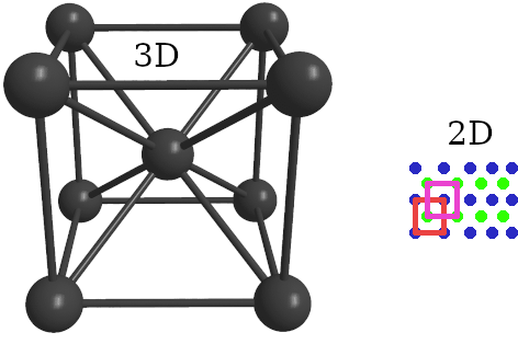 |
| bcc Structure |
The size of the \(F_e\) cubic struture is \(a=2.866 \) angstrom.
The interatomic spacing \(r_{ij}=\frac{\sqrt{3}}{2}.a \sim 2.480 \) angstrom.
The number of neighboring particles \(n_z=8\).
The Curie temperature is \(T_c=1043K\).
The spin wave MF correction \(\epsilon=0.766\).
The atomic spin moment \(\mu_s=2.22 \mu_B\).
By the definition of \(J_{ij}, J_{ij}=\displaystyle \frac{3 \times 1.3807 \times 10^{-23} \times 1043}{0.766 \times 8}=7.0510 \times 10^{-21}\)J/link. The anisotropy constant is \(k_u=5.65 \times 10^{-25}\).
The physical values can be summarized in the table:
| Variable | Symbol | Unit | Unit expression |
|---|---|---|---|
| Parameter | Symbol | value | Unit |
| Crystal structure | bcc | ||
| Atomic magnetic moment | \(\mu_s\) | \(2.22 \times \mu_B=2.058820 \times 10^{-23} \) | \(J.T^{-1}\) |
| Unit cell size | \(a\) | \(2.866 \times 10^{-10}\) | \(m\) |
| Interatomic spacing | \(r_{ij}\) | \(2.480\) | angstrom |
| Exchange Energy | \(J_{ij}\) | \(7.0510 \times 10^{-21}\) | J/link |
| Uniaxial anisotropic Energy | \(k_u\) | \(5.65 \times 10^{-25}\) | J/atom |
| Spin wave MF correction | \(\epsilon\) | \(0.766\) | - |
| Curie Temperature | \(T_c\) | \(1043\) | \(K\) |
Nickel element
The particles structure of the nickel ferromagnetic element \(N_i\) is a fcc struture. Each particle \(P_i\) is either at center of a face of a cube or at the summit of the cube. Each particle at the center of a face is connected to the particles at the summit of its face and to other particles at center of faces which are connected to its face. The number of neighboring particles is \(n_z=12\).
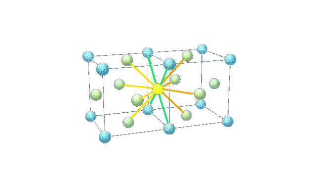 |
| fcc Structure |
The size of the \(N_i\) cubic struture is \(a=3.524\) angstrom.
The interatomic spacing \(r_{ij}=\frac{\sqrt{2}}{2}.a \sim 2.492 \) angstrom .
The number of neighboring particles \(n_z=12\).
The Curie temperature is \(T_c=631K\).
The spin wave MF correction \(\epsilon=0.790\).
The atomic spin moment \(\mu_s=0.606 \mu_B\).
By the definitition of \(J_{ij}, J_{ij}=\displaystyle \frac{3 \times 1.3807 \times 10^{-23} \times 631}{0.790 \times 12}=2.757 \times 10^{-21}\)J/link. The anisotropy constant is \(k_u=5.47 \times 10^{-26}\).
The physical values can be summarized in the table:
| Variable | Symbol | Unit | Unit expression |
|---|---|---|---|
| Crystal structure | fcc | ||
| Atomic magnetic moment | \(\mu_s\) | \(0.606 \times \mu_B=5.62\times 10^{-24} \) | \(J.T^{-1}\) |
| Unit cell size | \(a\) | \(3.524 \times 10^{-10}\) | \(m\) |
| Interatomic spacing | \(r_{ij}\) | \(2.492\) | angstrom |
| Exchange Energy | \(J_{ij}\) | \(2.757 \times 10^{-21}\) | J/link |
| Uniaxial anisotropic Energy | \(k_u\) | \(5.47 \times 10^{-26}\) | J/atom |
| Spin wave MF correction | \(\epsilon\) | \(0.790\) | - |
| Curie Temperature | \(T_c\) | \(631\) | \(K\) |
Variables normalization
The adimensioning of variables is done wthin the SM_Material class
The adimensionizing method consists in turning the physical variables with adimentionized variables :
- \(E=\bar e . e \)
- \(H=\bar h . h \)
- \(\tau=\bar t . t \)
- \(X=a . x\)
where \(X\) is a physical length value and \(x,e,h,t\) are adimensionized variables. For simplicity, as the cell size is a multiple of Angstrom, we take \(a=10^{-10}m=1\) angstrom and \(\mu_s=\tilde \mu_s . \mu_B \).
The adimensionizing LLG equation gives \( \displaystyle \frac{dS_i}{dt}=- \frac{\gamma}{1+\lambda^2} .\bar t . \bar h . \left (S_i \wedge h_{eff}^i + \lambda \left ( <S_i,h^i_{eff}> S_i - |S_i|^2. h^i_{eff} \right ) \right )\)
As \(\mu_s\) is chosen as a multiple of \(\mu_B\), we use:
from the equation of the dipolar energy \(\bar e= \mu_0 . \mu_B^2 . a^{-3}\) expressed in \(J\) and from the relation energt/magnetic field, \(\displaystyle \bar h = \frac{1}{\mu_B} \bar e\) expressed in \(T\)
So the characteristic physical value are by assuming that \(\gamma . \bar t . \bar h = 1 \):
\begin{eqnarray*} \bar e &= \mu_0 . \mu_B^2 . a^{-3} & J\\ \bar h &= \mu_0 . \mu_B . a^{-3} & T\\ \bar t &= \frac{a^3}{\gamma.\mu_0.\mu_B } & s\\ \end{eqnarray*}
The adimensionized correspondance of the relation energy/magnetic field :
\( \displaystyle h^i_{eff}=-\frac{1}{\tilde \mu_s}\frac{\partial e}{\partial S_i} \)
With this characteristic variables the LLG equation becomes:
\( \displaystyle \frac{dS_i}{dt}=\alpha \left (S_i \wedge h_{eff}^i + \lambda \left ( <S_i,h^i_{eff}> S_i - |S_i|^2. h^i_{eff} \right ) \right ) \)
with \(\alpha=-\frac{1}{1+\lambda^2}\).
The adimensionized external field \(h_{ext}\) is defined as:
\( h_{ext}=\displaystyle \frac{H_{ext}}{\bar h}=\displaystyle \frac{H_{ext}. a^3 }{\mu_0 . \mu_B } \)
The adimensionized Heisenberg field \(h_{exc}\) is defined as :
\( h_{exc}=\displaystyle \frac{H_{exc}}{\bar h}=\displaystyle \frac{1}{\tilde \mu_s}\sum_{ij} \tilde J_{ij} S_i \)
with \( \tilde J_{ij}=\displaystyle \frac{J_{ij}.a^3}{\mu_B^2.\mu_0} \)
The adimensionized DMI field \(h_{dmi}\) is defined as :
\( h_{dmi}=\displaystyle \frac{H_{dmi}}{\bar h}=\displaystyle \frac{1}{\tilde \mu_s}\sum_{ij} \tilde D_{ij} S_i \wedge S_j \)
with
\( \tilde D_{ij}=\displaystyle \frac{D_{ij}.a^3}{\mu_B^2.\mu_0} \)
The adimensionized anisotropy field \(h_{ani}\) is defined as :
\( h_{ani}=\displaystyle \frac{H_{ani}}{\bar h}=\displaystyle -\frac{1}{\tilde \mu_s }\tilde k_U \nabla \Phi_U(S_i) \)
with
\( \tilde k_u= \frac{k_U.a^3}{\mu_B^2 .\mu_0} \)
The adimensionized dipolar Energy \(e_{dip}\) is defined as :
\begin{eqnarray*} e_{dip}&=&\displaystyle \frac{E_{dip}}{\bar e} \\ &=&\frac{\mu_0\mu_B^2.\tilde \mu_s^2}{4.\pi a^3} \frac{a^3}{\mu_0.\mu_B^2} \sum_{j\neq i} \frac{1}{\tilde r_{ij}^3}<S_i,S_j> - \frac{3<S_j,\tilde r_{ij}>_3}{\tilde r_{ij}^5} < \tilde r_{ij},S_i> \\ &=&\displaystyle \frac{\tilde \mu_s^2}{4.\pi} \sum_{j\neq i} \frac{1}{\tilde r_{ij}^3}<S_i,S_j> - \frac{3<S_j,\tilde r_{ij}>_3}{\tilde r_{ij}^5} <S_i,\tilde r_{ij}> \label{Eq.AEdip} \end{eqnarray*}
with \(\tilde r = \displaystyle \frac{r}{a}\) expressed in ansgtrom.
By the adimensionized relation between energy and magnetic field, the adimensionized dipolar field is
\( h^i_{dip}=\displaystyle - \frac{\tilde \mu_s}{4.\pi} \sum_{j\neq i} \frac{1}{\tilde r_{ij}^3}S_j - \frac{3<S_j,\tilde r_{ij}>_3}{\tilde r_{ij}^5} \tilde r_{ij} \)
The characteristic values do not depend on the material:
| variable | Characteristic Values | expression | value | unit |
|---|---|---|---|---|
| time | \(\bar t\) | \(\frac{a^3}{\gamma.\mu_0.\mu_B }\) | \(4.8754 \times 10^{-13}\) | \(s\) |
| energy | \(\bar e\) | \(\mu_B^2 . \mu_0 . 10^{-30} \) | \(1.0808\times 10^{-22}\) | \(J\) |
| field | \(\bar h\) | \(\mu_B . \mu_0 . 10^{-30} \) | \(11.6541\) | \(T\) |
The adimensionized values for the Fe material are :
| Adimensionized Values | expression | value |
|---|---|---|
| \(\tilde J_{ij}\) | \(\displaystyle \frac{J_{ij}.10^{30}}{\mu_B^2.\mu_0}\) | \(65.2388\) |
| \(\tilde k_u\) | \(\displaystyle \frac{k_U. 10^{30}}{\mu_B^2 .\mu_0}\) | \(0.00522761 \) |
With respect of the small value of characteristic energy, it is more pertinent to use the adimensionized formulation of the system when energy is used for using convergence criterium because its variation is too small to be detected by computation.
Numerical temperature modelization
The Landau-Lifschitz equation can be rewritten as follow :
\( \displaystyle \frac{d\mu}{dt}=\alpha. A(\mu) h \)
where \(A: \mathbb{R}^3 \rightarrow M_{3\times3} \) is defined by
\( \displaystyle A(x)=L(x) + \lambda ( x.x^t - x^t.x I ) \)
and
\begin{eqnarray*} \displaystyle L((x_1,x_2,x_3))=\begin{pmatrix} 0 & -x_3 & x_2 \\ x_3 & 0 & -x_1 \\ -x_2& x_1 & 0 \end{pmatrix} \end{eqnarray*}
Thermal effect
In order to model thermal effects, a stochastic perturbation is introduced. Thermal effect can be embedded in the deterministic system by adding a stochastic perturbation to the field h by considering a standard F-Brownian motion which leads to the following stochastic system
\( \displaystyle d\mu=\alpha. A(\mu_t) h.dt + \epsilon \alpha A(\mu_t)dW_t \)
Stratonovich approach
This numerical model is implemented within SM_LandauLifschitzSystem and its implementations SMOMPI_StratonovichSystem and SMOMPI_StratonovichNormalizedSystem .
In order to preserve the norm of S , the Stratonovich approach consists in adding a new term \( K_t . dt \) in the stochastic equation and choosing \( K_t \) such that \( d|\mu_t|=0 \).
We recall the ito theorem:
Let's denote by \( W \) a brownian movement in \(R^d \) and
\[ \begin{array}{lll} Xt &:& R \rightarrow R^n \\ & & t \mapsto X_t \\ b &:& R^+ \times R^n \rightarrow R^n \\ & & (t,X) \mapsto b(t,X) \\ \sigma &: & R^+ \times R^n \rightarrow R^n\times R^d \\ & & \displaystyle \partial X_t=b(t,X_t).dt + \sigma(t,X_t) dW_t\\ \end{array} \]
if we note by
\[ \begin{array}{lll} f &:& R^+ \times R^n \rightarrow R \\ & & (t,x) \mapsto f(t,X)\\ \end{array} \]
we have
\( df(t,X_t)=\displaystyle \frac{\partial f}{\partial t} dt + \nabla_xf(X_t).dX_t +\frac{1}{2} \sum_{i,j} \frac{\partial^2 f(t,X_t)}{\partial x_i \partial x_j} .d<x_i,x_j>_t \)
with \(d<x_i,x_j>_t=(\sigma(t,X_t).\sigma(t,Y_t)^T)_{ij} dt \)
By Appliing the Ito theorem to \(f(t,X)=<X,X>\) with \(d\mu_t\) verifiing \(\displaystyle d\mu_t=\alpha. A(\mu_t) h.dt + \epsilon \alpha A(\mu_t)dW_t + K_tdt\),
\(d|\mu_t|^2=2<\mu_t,\alpha.A(\mu_t).h dt+ \epsilon \alpha A(\mu_t)dW_t + K_tdt>+\frac{1}{2}. \sum_{i,j} 2.\delta_{ij}.\varepsilon^2.\alpha^2.A(\mu_t).A(\mu_t)^T dt\)
As we have from LL equatiob that \(<d\mu_t,\alpha.A(\mu_t).h dt+ \epsilon \alpha A(\mu_t)dW_t>=0\), we conclude that
\(d|\mu_t|^2=2.<\mu_t,K_t>.dt + \varepsilon^2.\alpha^2 . tr(A(\mu_t).A(\mu_t)^T)dt\)
After some computations, we have
\(tr(A(\mu_t).A(\mu_t)^T)=2|\mu_t|^2+3\lambda^2|\mu_t|^4-2\lambda^2|\mu_t|^4+\lambda^2|\mu_t|^4\)
So \( d|\mu_t|^2=\displaystyle 2. \varepsilon^2.\alpha^2.dt.|\mu_t|^2.\left( 1+\lambda^2.|\mu_t|^2\right)+2.<\mu_t,K_t>.dt\)
To have a null variation of the norm of \(\mu\), we can impose that
\( K_t= - \varepsilon^2.\alpha^2.dt.|\mu_t|^2.\left( 1+\lambda^2.|\mu_t|^2\right) \cdot \mu_t \)
So the Stratonovich equation becomes with with \(|\mu_t|=1 \),
\( \displaystyle d\mu_t=\alpha. A(\mu_t) h.dt+ \epsilon \alpha A(\mu_t)dW_t - \varepsilon^2.\alpha^2.\left( 1+\lambda^2\right).dt.\mu_t \)
We can assume now that the noise rate \(\varepsilon\) may be dependant on t. It will be denoted by \(\varepsilon_t\).
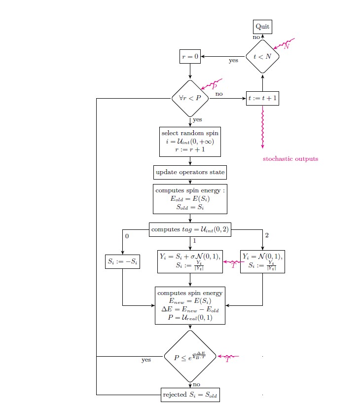
The algorithm is as follow for the stratonovich or Ito algorithm ( \(\tau=0\) for Ito algorithm)
- 1. initializes the seed of the stochastic function
- 2. initializes to zero, the mean of \(\mu, \bar \mu=0\)
- 4. for each trajectory s in [0,S[ do
- 4.0 initializes \(t=0\)
- 4.1 computes \(h=h_{ext}^t+h_{exc}^t+h_{ani}^t+h_{dip}^t\) the Zeeman, Heissenberg, anisotropy, and dipolar magnetic fields at time t
- 4.2 computes the time step \(dt\) (regular for the version 0.03)
- 4.3 computes the Brownian motion number \(dW_t \sim \displaystyle \sqrt{dt}.\mathcal{N}(0,1)\)
- 4.4 computes \(dh=h.dt+\varepsilon_t.dW_t\)
- 4.5 computes the normalisation rate \(\tau=\varepsilon_t^2.\alpha^2.\left( 1+\lambda^2\right).dt \)
- 4.6 computes \(\mu_{t+dt}=(1-\tau).\mu_t+LL(\mu_t,dh)\)
- 4.7 normalizes \(\mu_{t+dt}\) if needed
- 4.8 goes to step 4.1 with \(t:=t+dt\), \(\mu_t:=\mu_{t+dt}\) while \(t<T\)
- 6. go to 4.0 while s < S
Numeric errors impose that the step 4.7 must be done. if not, the algorithm does not converge numerically.
\(\forall t \in [0,T_{target}], \mu(s,t)\) are computed by the Stratonovich system algorithm can be illustrated as follow:

Heun Algorithm
This numerical model is implemented within SM_LandauLifschitzSystem and its implementations SMOMPI_HeunSystem .
In the Heun method, the predictor step calculates the magnetic moment \(\mu_t^p\) from \(\mu_t\), \(h_t\) and a generated Brownian motion \(dW_t\) by integration step:
\begin{eqnarray*} dW_t &=& \sqrt{dt}.\varepsilon. \mathcal{N}(0,1) \\ h_t &=& h_{ext}(\mu_t)+h_{exc}(\mu_t)+h_{ani}(\mu_t)+h_{dip}(\mu_t) \\ dh_t &=& dt.h_t+dW_t \\ \Delta \mu_t^p &=& LL(\mu_t,dh_t) \\ Y &=& \mu_t+\Delta \mu_t^p \\ \forall X , \mu_t^p(X) &=&\frac{1}{|Y(X)|_3} Y(X) \\ \end{eqnarray*}
where \(X\) is the particle position. After the predictor step, the effective field must be re-evaluated as the intermediate spin positions have now changed. The Brownian motion is those computed at the predictor step. The corrector step uses the predicted spin position and revised effective field to compute the final spin position at next time \(t+dt\):
\begin{eqnarray*} h^c_t&=&h_{ext}(\mu_t^p)+h_{exc}(\mu_t^p)+h_{ani}(\mu_t^p)+h_{dip}(\mu_t^p) \\ dh^c_t &=& dt.h^c_t+dW_t \\ \Delta \mu_t^c &=& LL(\mu^p_t,dh^c_t) \\ Y &=& \mu_t+\frac{1}{2} \left (\Delta \mu_t^p + \Delta \mu_t^c \right ) \\ \forall X , \mu_{t+dt}(X) &=& \frac{1}{|Y(X)|_3} Y(X) \\ \end{eqnarray*}

Monte Carlo Algorithm
This numerical model is implemented within SM_MonteCarloSystem and its implementations SMOMPI_MonteCarloSystem.
For having a comparison method, the classical Monte Carlo Metropolis algorithm is used.
It consists in picking up randomly a spin \(i\) and its initial spin direction \(S_i\) is changed randomly into a new direction \(S^{'}_i\).
The change in energy \(\Delta E = E(S^{'}_i)-E(S_i)\) is computed and the new position is accepted with the probability \(P=e^{-\frac{\Delta E}{k_B.T}}\).
The procedure is repeated P times where \(P\) is the number of spins. Each set of \(P\) spin moves is 1 step.
The randomly move of a spin is either
- a flip move: \(S^{'}_i=-S_i\) or
- a gaussian move: \(Y_i=S_i+\sigma. \mathcal{N}(0,1), S^{'}_i=\frac{Y_i}{|Y_i|}\) with \(\sigma=\frac{2}{25}.\left( \frac{T.k_B}{\mu_B} \right)^{\frac{1}{5}}\)
- a random move: \(Y_i=\mathcal{N}(0,1), S^{'}_i=\frac{Y_i}{|Y_i|}\).
The algorithm is as follow for 1 simulation where N is the number of steps and P the number of spins:
Temperature and noise rate modeling
This model is implemented within SM_TemperatureNoiseRate
The thermal effect is modelized by the instantaneous thermal field on spin at particle \(i\) by
\[ H_{th}=\displaystyle \varepsilon_t . \mathcal{N}(0,1) \]
where \(\mathcal{N}\) is the Gaussian distribution of mean of zero and of standart deviation of 1 and \(\varepsilon_t\) in Tesla unit. The link between time independant \(\varepsilon_t=\varepsilon\) and the temperature is
\[ \varepsilon=\displaystyle \sqrt{\frac{2\lambda.k_B.T}{\gamma . \tilde \mu_s . \mu_B . \bar t }} \]
where \(k_B\) is the Boltzmann constant, \(T\) is the system temperature, \(\lambda\) is the Gilbert damping parameter and \(\gamma\) is the absolute value of the gyromagnetic ration, \(\mu_s\) is the magnitude of the atomic magnetic moment normalized by \(\mu_B\) and \(\bar t=\frac{10^{30}}{\gamma . \mu_0 \mu_B }\) is the characteristic time.
With the characteristic magnetic values \(\bar t =\frac{10^{-30}}{\gamma \mu_0.\mu_B}\), we have
\begin{eqnarray*} \displaystyle \varepsilon &=& \displaystyle \sqrt{\frac{k_B\mu_0}{A^3}} \sqrt{\frac{2.\lambda.T}{\tilde \mu_s}}\\ &\sim& 1.644561 \sqrt{\frac{2.\lambda.T}{\tilde \mu_s}} \end{eqnarray*}
Parallel implementation
To improve the CPU time performance, the code is parallelized with
- OpenMP: the computing loop on particles of the network is divided in slice of particles of same size for each core.
- mpic: the whole network and the direction of the spins are distributed to all cores. Each core computes its own slice of particles and the whole field is gathered and send to all cores.
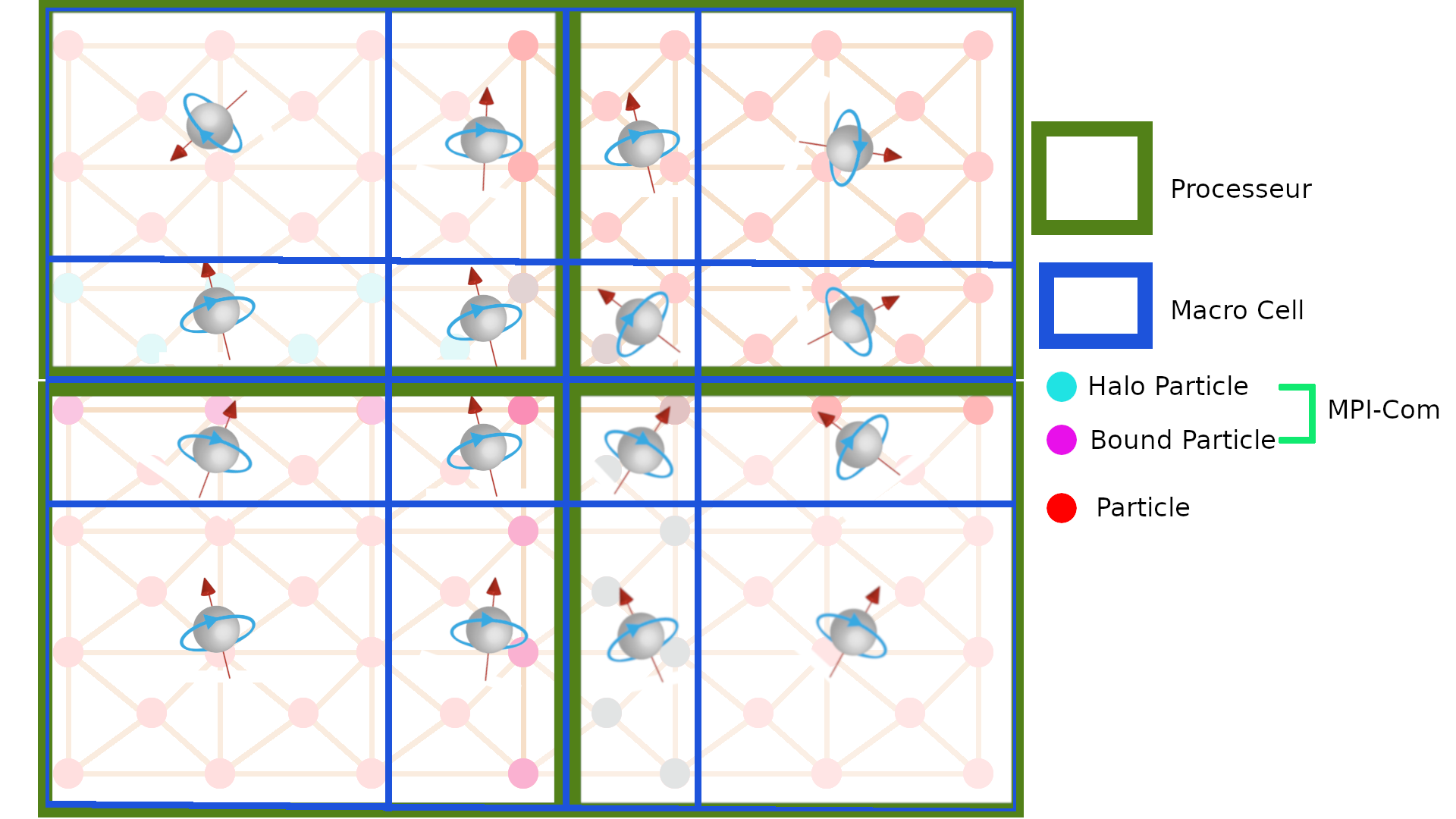
- mpi: the whole network is divided in block parts. Each part of network is managed by its own core. The data values on holes & bounds particles are exchanged between cores.
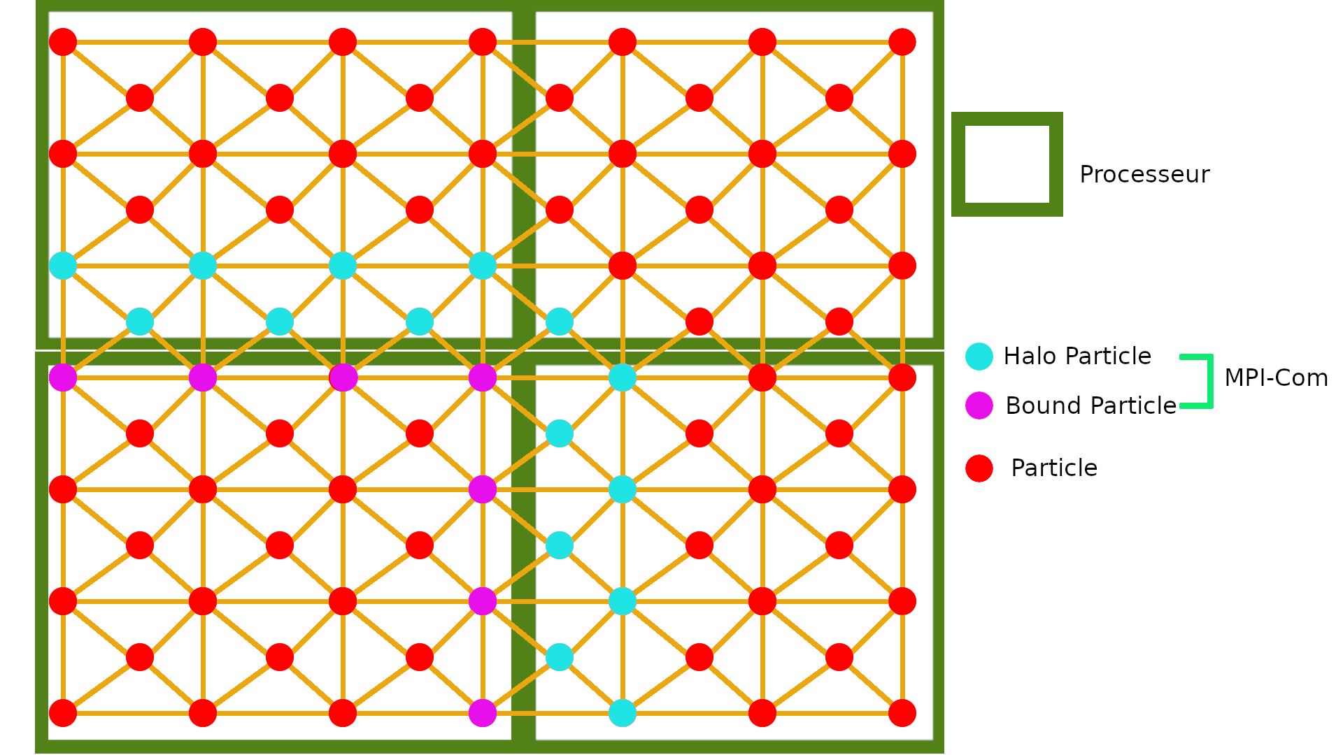
mpi parallelization
A core \(C_i\) has neighbor cores \(C_{j}\). The set of halo particles of the core \(C_i\) is divided with respect of the core \(C_j\) to which its belongs.
An halo particle \(P_{h}\) belongs to only one core \(C_j\). The halo particle is link to bound particles \(P_b\). A bound particle may be shared with several cores \(C_j\). The mpi communications are :
- the core \(C_i\) sends the bound particles of \(C_j\) of its network into the halo particles of network of core \(C_j\) belonging to network of core \(C_i\)
- the core \(C_i\) received all the bound particles of network of core \(C_j\) into the halo particles of its network belonging to core \(C_j\). We illustrate the bound and halo particles for bottom left core :
 |
| macro cells |
This communication is necessary for computing the Heisenberg/DMI operators which need to know the spin direction of the halo particles.
A block \(B_I\) of the network blocks decomposition is defined by its min point \(P_I\) and max point \(Q_I\). All the particles in \([P_I,Q_I[\) belongs to the network of the core \(B_I\) (one core per block, the network as \(B\) blocks). For convenience, a margin \(\varepsilon \in R^3\) is added in order to be sure that a particle is not at the boundary of two blocks. \(P_0=-\varepsilon\) and \(Q_B=Q+\varepsilon\) when \(Q\) is the max point of the network.
The number of blocks depends on the number of avaliable cores: \(N_{cpu}=N_{cpu}^x . N_{cpu}^y . N_{cpu}^z \).
The number of blocks per direction is defined to minimize the surface of the block of the core divided by its volume. If \(L\) denotes the length of the grid per direction, the surface of the block is:
\( S= 2 \left ( \frac{L^x.L^y}{N_{cpu}^x.N_{cpu}^y}+\frac{L^y.L^z}{N_{cpu}^y.N_{cpu}^z}+ \frac{L^z.L^x}{N_{cpu}^z.N_{cpu}^x} \right ) \)
The volume of the block is \(V=\frac{L^x}{N_{cpu}^x}.\frac{L^y}{N_{cpu}^y}.\frac{L^z}{N_{cpu}^z}\).
To compute the minimum of \(\frac{S}{V}\), the set \(\vartheta \) of all the divisors of \(N_{cpu}\) is computed and all the combinaisons of \(N^k_{cpu} \in \vartheta, \forall k \in \{x,y,z\}\) is tested to select the minimum of \(\frac{S}{V}\).
This network is implemented in the class SM_Network
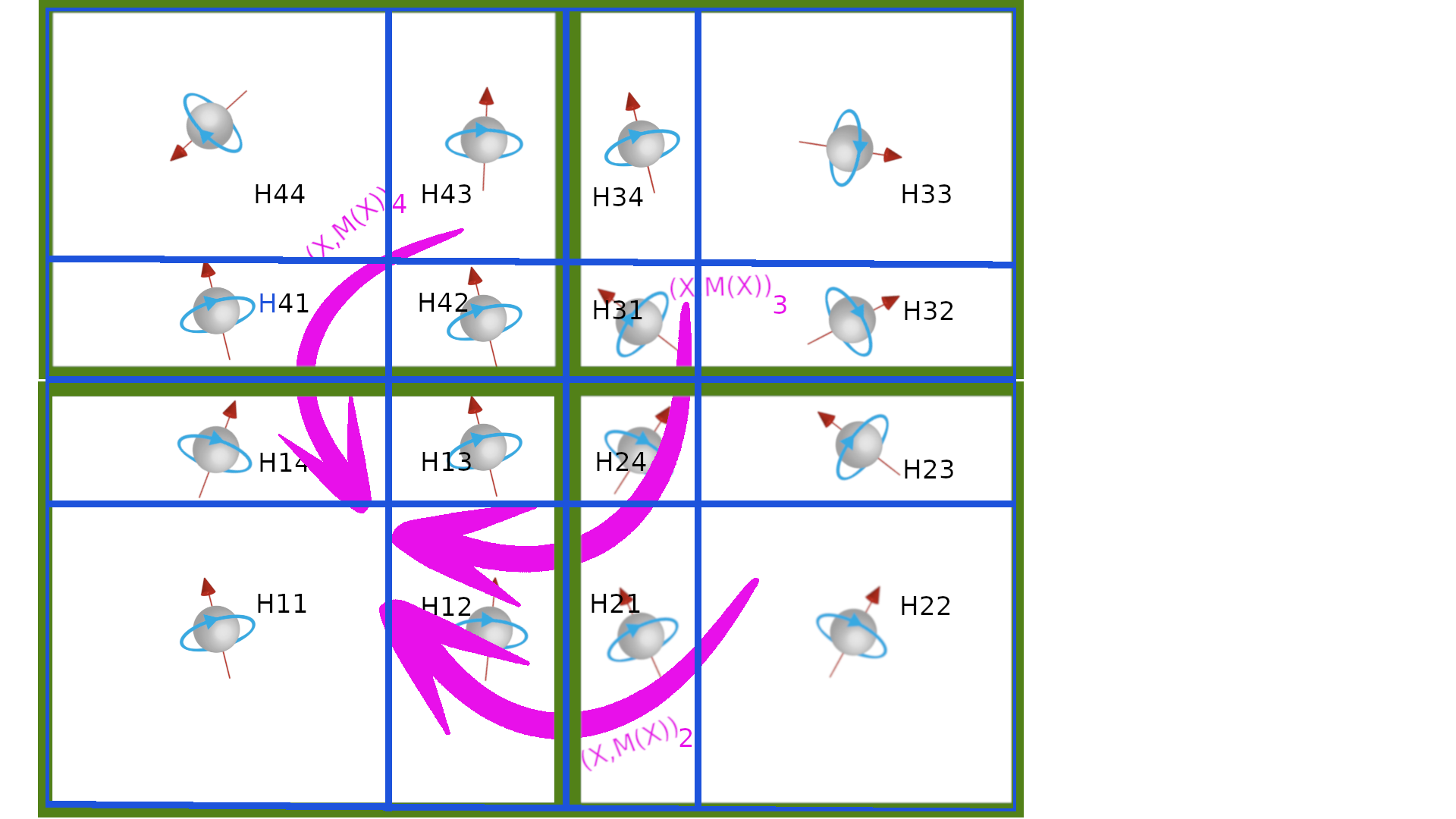
mpi parallelization for Demagnetized field
For the demagnetized operator, its is more complicated because the demagnetized field needs to the the mass center and the magnetization at all macro cells of its neighbor cores. The macro cells network is composed by a grid of macro cells m. The mass center \(X^m\) of the macro cell \(m\) is the magnetic barycenter of the position of particles in the macro cell m whose weight is the magnetic moments. The magnetization field \(M^m\) applied on the mass center of the macro cell is the sum of magnetic moment of spins included in the macro cell
 |
| macro cells |
3 strategies are used to solve the problem:
- All-Master : each core owns the macro cells data ( \(X^m,M^m,H_{dem}^m\)) over the whole macro cells grid. Each core computes the demagnetized field \(H_{dem}\) within a slice of the macro cell grid. Then, each core gathers \(H_{dem}\) from the slices of the all other cores.
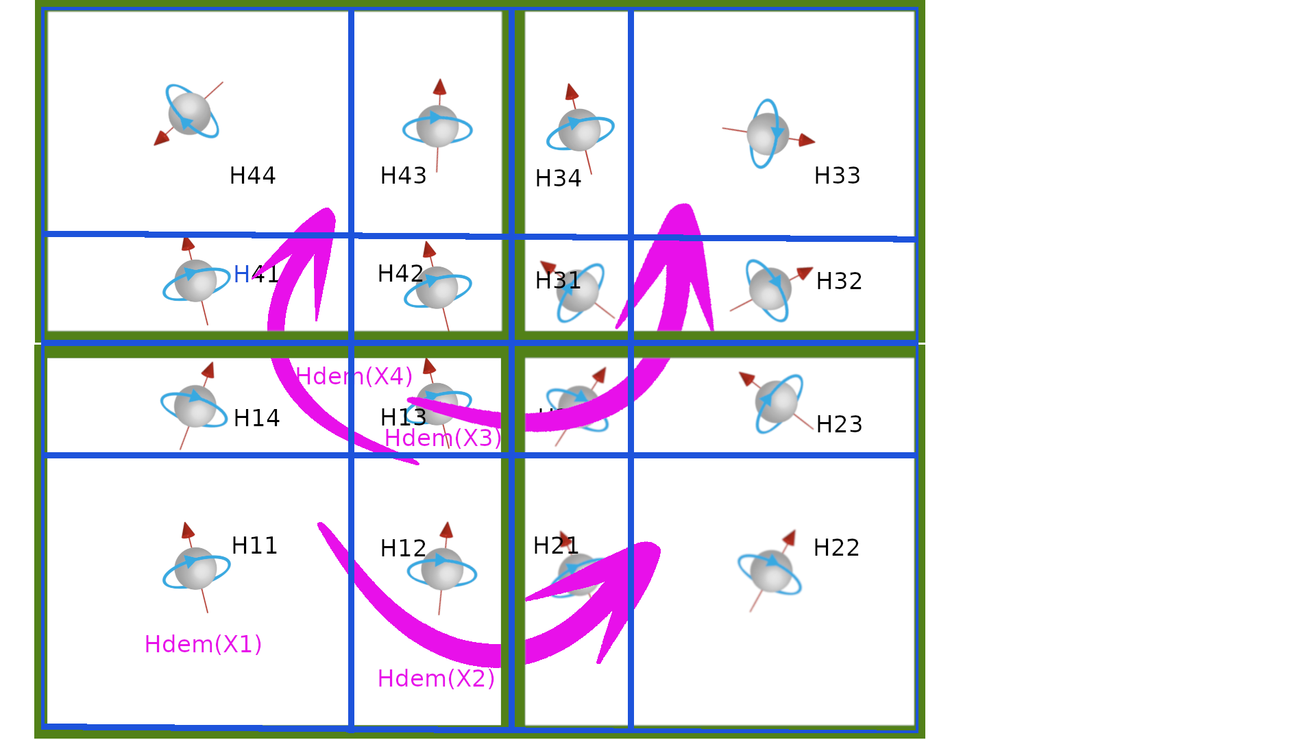
- One-Master : each core \(c\) owns the macro cell data only on the macro cells which contain a particle of the network of the core \(c\). A master core gathers the macro cell data by a variable sum reduction over the other cores in order to compute \(H_{dem}\) on the whole macro cells grid. Finaly, the master core scatters the demagnetized field to all other cores.
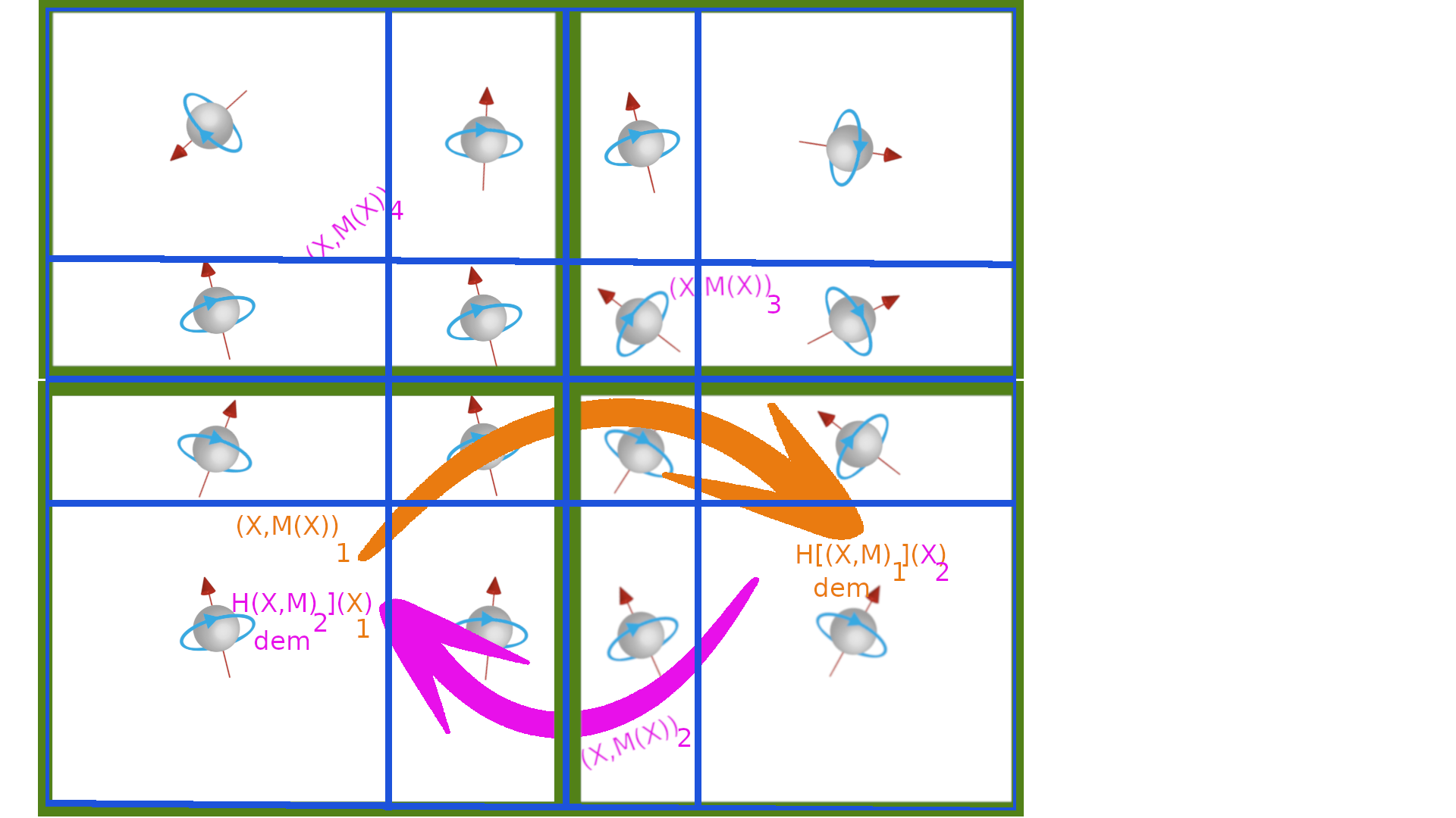
- No-Master: each core has its own macro cells grid which are not shared with other cores. Each core sends to other core its macro cell data to compute the demagnetized field on the macro cells within its own macro cells grid. In this case, the macro cell size is not uniform over the macro cells network.
all master cores communication
Each core c computes its own contribution into the macro cells network data of size \(N^{mc}\):
- \(N^m\) of size \(N^{mc}\), is number of particles in macro cell m
- \(X^m\) of size \(3 \times N^{mc}\) : sum of the particles position in macro cell m
- \(M^m\) of size \(3 \times N^{mc}\) : sum of the particles magnetic moment in macro cell m
The total number of particles in macro cell \(m\) is the sum of the particles number of the network of cores computed by mpi-sum-all-reduction over a fixed size array.
The mass center \(C^m=\frac{X^m}{N^m}\) of each macro cell \(m\) is the mean sum of position of particles of the network of cores. It is another mpi-sum-all-reduction over a fixed size array.
The magnetization field of a macro cell \(m\) is the sum of the magnetic dierction of particles of the network of cores. It is another mpi-sum-all-reduction over a fixed size array.
Each core computes the demagnetized field over a slice of the macro cells grid and gathers all the slices from the other cores of the demagnetized field into the \(H_{dem}\) field defined on the whole macro cells grid.
This method ensures that the macro cell size is constant.
\( (N^m,X^m,M^m) \xrightarrow[]{\text{All Reduce}} (N^m,X^m,M^m) \xrightarrow[\text{in core c}]{\text{compute}} H^m_{dem}(C^m,M^m)[C^{m \in slice_c}] \xrightarrow[]{\text{All Gather}} H^m_{dem} \)
one master core communication
Each core c computes the macro cells network data whose macro cell owns at last on particle of the network of the core. The number of macro cells of the core c is \(N^{mc}_c\)
- \(N_c^m\) of size \(N^c_{mc}\), is number of particles in network of core \(c\) and in macro cell m
- \(X_c^m\) of size \(3 \times N^c_{mc}\) : sum of position of the particles of core \(c\) in macro cell m
- \(M_c^m\): sum of the magnetic moment of particles in core \(c\) and in macro cell m
- \(I_c : [0,N^{mc}_c[ \mapsto [0,N^{mc}[\) is the map from the index of macro cell in the macro cells network of core c to its corresponding index in the whole macro cells network.
- \(H_{dem,c}^m\) of size \(3 \times N_{mc}^c\) : demagnetized field on macro cells into the core c.
Each core c sends \((I_c,N_c,X_c,M_c)\) to a master core \(c_m\) to gather the macro cells network data \((N^m,X^m,M^m)\) of the whole macro cells network within by master core \(c_m\) in order to build \(C^m=\frac{X^m}{N^m}\). The demagnetized field \(H_{dem}(C^m)\) is computed and scattered to all other cores into \(H_{dem,c}^m\)
\( (I^m,N^m,X^m,M^m)_c \xrightarrow[\text{to core $c_m$}]{\text{Gather}} (N^m,X^m,M^m) \xrightarrow[\text{in core $c_m$}]{\text{compute}} H^m_{dem}(\frac{X^m}{N^m},M^m) \xrightarrow[\text{to core c}]{\text{scatter}} H^m_{dem,c} \)
 |
 |
| receive | send |
no master communication
Each core c computes its own macro cells grid. The number of macro cells of the grid of the core c is \(N^{mc}_c\)
Each core \(c_i\) receives \((C,M)_j\) from all other cores \(c_j\). When the data are received, the demagnetized field from macro cells on \(c_j\) is computed \(H_{cdem,_i}(C_i)+=H^{dem}_{(C_j,M_j)}(C_i)\). The cpu time for communication is supposed to be compensated by the computation time.
\( (C,M)_i \xrightarrow[\text{from core $c_j$}]{\text{receive}} (C,M)_j \xrightarrow[\text{in core c_i}]{\text{compute}} H_{dem}(C_j,M_j)[C_i] \)
 |
| receive and compute |
In that case the size of macro cells is not necessarly uniform.
mpi parallelization for numerical algorithms
Parallel Landau Lifschtiz System
The parallel algorithm for the landau lisfchitz system is almost the same as the serial algorithm. One step is added : after computing the directions of the magnetic moment of all spins at next time step, the direction of magnetic spin of halo particles \( p_h \) of a core i must be set to its corresponding bound particle \(p_b\) within neighbor core j. The core j sends the values on particles \(p_h\) to the core i which receives them for the corresponding particle \(p_h\).
\( S^{c_i}_{t+dt}(p_h)=S^{c_j}(t+dt)(p_b) \)
parallel metroplis Monte Carlo System As in parallel Landau Lifchitz system, one step is added: after computing the directions of the magnetic moment at next simulation, the direction of magnetic spin of halo particles of a core i must be set to its corresponding bound particle within neighboring core j . Nothing particular is done for the steps of one simulation.
parallel beam algorithm
In parallel, for the mpi version, the beam simulation is not parallelelized: all system do the same number of simulations. A synchronisation is automatically done after exchanging mpi data between halo and bound particles.
For the version hybrid openmp-mpi version, te parallel simulations consists in dividing the S simulations by the number of cores \(N_{cores}\).
Let's note \(\forall c \in [1,N_{cores}], s_c=c. \frac{S}{N_{cores}}\).
Each core \(c \in [1,N_{cores}]\) runs \(s_{c-1}-s_c\) simulations.
To satisfy the generated random numbers per each core to be independent one from the others, a stochastic jump is applied to the stochastic function.
The number of simulated random numbers (a jump) is the number of random numbers generated by a simulation multiply by the number of simulations done for all cores whose id is less that c : jump= \(N_{rng} \cdot s_{c-1}\)
If the stochastic function has not an integrated jump function, each core c initializes the seed of its stochastic function by generating c uniform random integer numbers and by taking the last generated random number:
\( \forall i \in [0,c[ jump=\mathcal{U}_{int}([0,+\infty[)\)
The mpi implmentations is done oin mpi package version of each package which needs to be parallelized.
Beam simulation
The beam simulation, done by the class SM_Beam, consists in running S simulations where one simulation is divided in 2 parts:
- a preconditionning part to reach a stabilization state from initial state \(S(t=0)\) for \(t_r\) steps.
- a statistic part to compute the statistic data for \(t_s\) steps.
It can be illustrated at follow:
The beam simulation, done by the class SM_Beam , can be illustrated as follow:
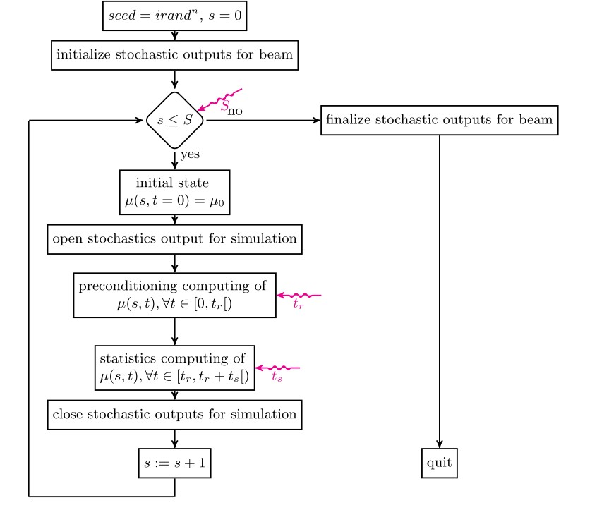
The corresponding algorithm of a beam to generate stochatic outputs is as follow:
- outputSData.close(SM_Beam)
- \( \forall s \in [s_0,s_1[ \) do
- SM_System::initializeMagnetMomentDirections()
- SM_StochastOutput::open(s,SM_System)
- ok=SM_System::stochastocRun(mPreconditioningStepsNumber,SM_MultiStochasticFunctionsInterface)
- ok=ok && SM_System::stochastocRun(mPreconditioningStepsNumber,SM_MultiStochasticFunctionsInterface,SM_StochastOutput)
- SM_StochastOutput::close(s,SM_System,ok)
- outputSData.close(SM_Beam)
It is possible to simulate a cycle of beam : each step of the cycle modified a parameter of the system to compute the beam simulation. The cyle algorithm is as follow
