 |
 |
 |
 |
 |
 |
 |
 |
 |
 |
 |
|
|
|
|

|

|
|
|

|
| Home | Gallery | CV | Visit | Publications |
Branched Transport
in collaboration with F. Santambrogio
We present on this page some preliminary results on optimal irrigation problems obtained in collaboration with Filippo Santambrogio. We refer to A Modica-Mortola approximation for branched transport and applications for additional details. Such optimal irrigation networks received a large attention last years (see for instance the articles of Xia, Bernot, Maddalena, Morel, Santambrogio and Solimini). Many qualitative results and generalization of the problem have been discussed. Nevertheless, it is surprising that very few has been done on the numerical approximation of optimal networks. One explanation is given by the fact that the exact identification of global optimal networks, in the combinatorial context (see below), is known to be NP hard (with respect to the number of dirac measures).
|
In order to tackle this difficulty we introduced a new continuous framework based on a  -convergence result obtained recently by F. Santambrogio which leads to a very efficient numerical procedure. Let us introduce first this kind of problem in a discrete setting. Consider a compact convex domain
  and two measures which are sum of dirac masses :
![\[ s = \sum_{i=1}^m a_i \,\delta_{x_i} \,\, \text{and} \,\, g = \sum_{j=1}^n b_j \, \delta_{y_j} \]](form_2.png)
where  and
and  are positive numbers. We ask to
  and
and  to have the same total mass, that is
  . Following Xia, we define a transport path
  from to as both a weighted directed graph $G$ which vertices contains the points
  and
and  and a weight function
  where
where  is the set of directed edges of
  . Moreover we ask
  to satisfy Kirchhoff's law that is for all vertex
  of we have:
![\[ \sum_{e\in E(G),\, e^- = v} w(e)= \sum_{e\in E(G),\, e^+ = v} w(e) + \left\{ \begin{array}{rl} \displaystyle a_i & \text{if $v = x_i$ for some} \; i\\ -b_j & \text{if $v = y_j$ for some} \; j \\ 0 & \text{otherwise} \end{array} \right . \]](form_16.png)
where  and
and  denote the starting and ending points of each directed edge
  . To every transport path we associate a cost of transportation defined by
![\[ M_{\alpha}(G) = \sum_{e\in E(G)} w(e)^\alpha \;\text{length}(e) \]](form_20.png)
for some fixed parameter ![$\alpha \in [0,1] $](form_21.png) .
.
 |
 |
 |
 |
 |
 |
 |
 |
 |
 |
We recall below how this discrete problem can be translated in a continuous context and the main -convergence obtained by F. Santambrogio. Let be a transport path associated to the two measures and . In order to introduce a relaxed formulation to the previous problem we associate to every the vectorial measure
![\[\displaystyle u_G = \sum_{e \in E(G)} w(e) \, \frac{e^+ - e^-}{||e^+ - e^-||} \mathcal{H}^1_{\vert e}.\]](form_22.png)
By definition, the measure  is in the class of vectorial measures of the type
  , where
  and
and  are respectively a positive function and a unit vector field defined on
  a set of finite
  -Hausdorff measure. Moreover Kirchhoff's law in this continuous setting is equivalent to the divergence constraint
![\[\nabla . u = g - s.\]](form_29.png)
In a analogous way to (costalpha}) we define for every vectorial measure the cost functional:
![\[ M^\alpha (u) = \left\{ \begin{array}{l} \int_M \theta ^\alpha \, d \mathcal{H}^1 \; \text{if $u$ is of the type $u(M,\theta,\xi)$ } \\ + \infty \;\;\text{otherwise} \end{array} \right . \]](form_30.png)
Thus, our relaxed optimisation problem is to minimise  under the previous (weak) divergence constraint. The -convergence result we are going to present is based on functionals very similar to the ones of Modica and Mortola but of the form
![\[ \displaystyle E_\varepsilon(u) = \varepsilon^{\gamma_1} \int _\Omega | u|^\beta + \varepsilon^{\gamma_2} \int _\Omega |\nabla u|^2\]](form_32.png)
defined on  with
with  . The main difference with Modica and Mortola's functionnal is the fact that the double-well potential has been replaced by a concave power
  which forces the modulus of the vector field to tends to
  or
or  . The idea is now to choose the parameters
  ,
,  and to obtain a functional equivalent (asymptotically when
  tends to ) to the cost (costcont}). Considering that the support of is concentrated on a segment, an heuristic argument leads to the following choice of the parameters :
![\[ \beta = \frac{2-2N + 2 \alpha N}{3-N + \alpha(N-1)},\;\;\frac{\gamma_1}{\gamma_2}=\frac{(N-1)(\alpha-1)}{3-N + \alpha(N-1)} \]](form_41.png)
Let us call  the functional associated to a set of parameters satisfying conditions (paramirrig}). F.
 : Suppose
  and
and ![$\alpha \in ]1/2,1[$](form_45.png) . Then -converges to
. Then -converges to  with respect to the convergence of measures for some suitable constant
  when tends to .
The previous -convergence result makes it possible to replace an hard discrete problem by a sequence of optimisation problems under linear constraints. In addition, we observed that for  the functional is close from being convex. This observation was the starting point of our optimisation strategy. The main difference between this situation and the previous one is related to the divergence constraint. Due to the very simple structure of the constraints we had to deal with, it was straightforward to compute a projection on the linear constraints in the context.
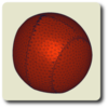
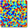
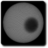
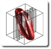
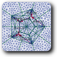
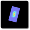
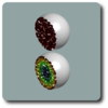
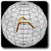
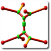
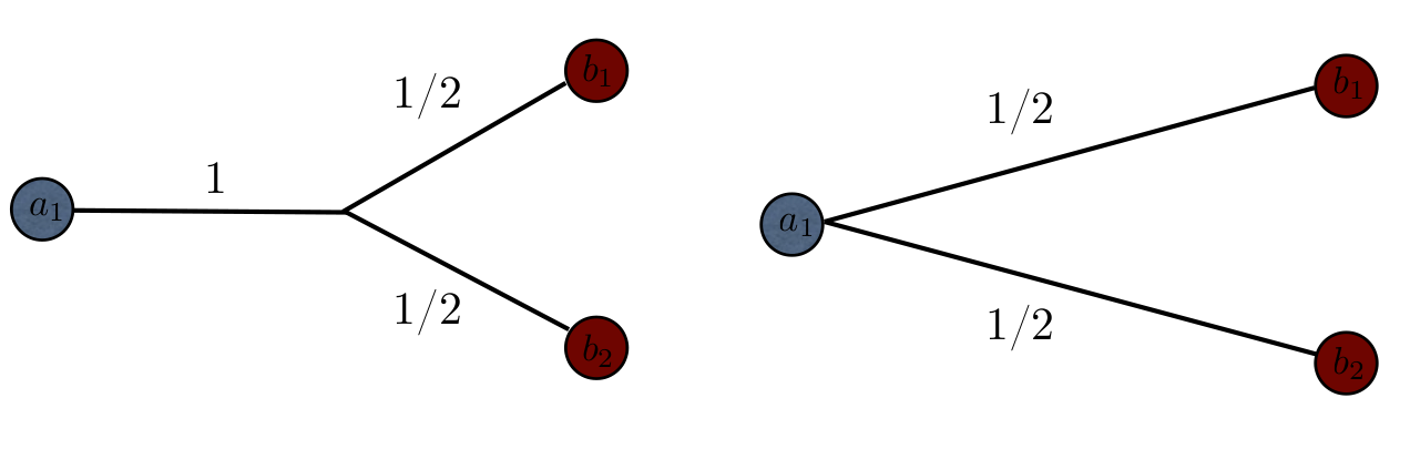
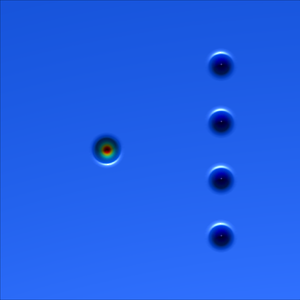
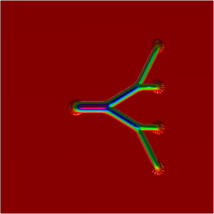
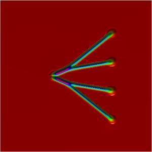
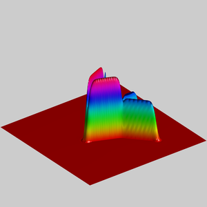
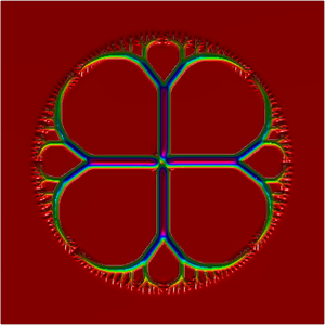
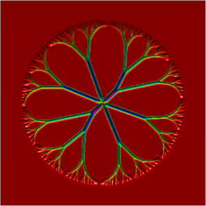
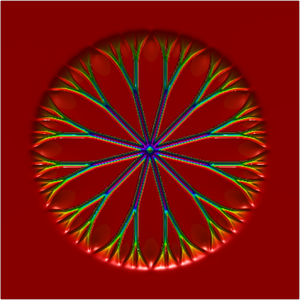
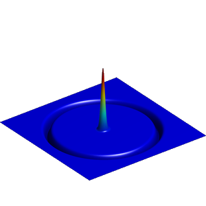
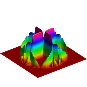
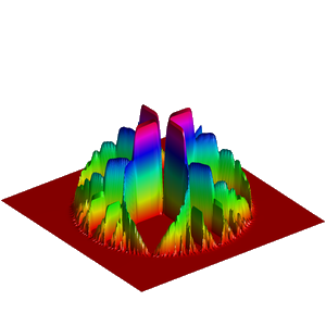
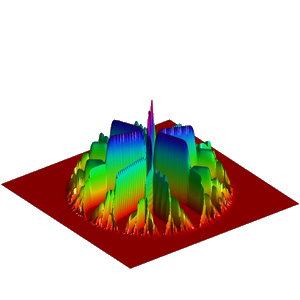
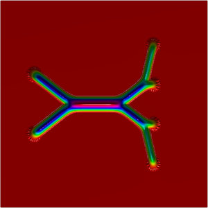
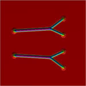
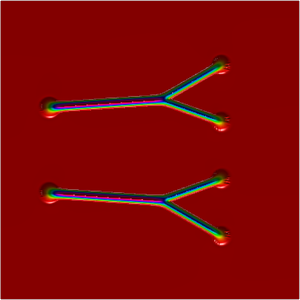
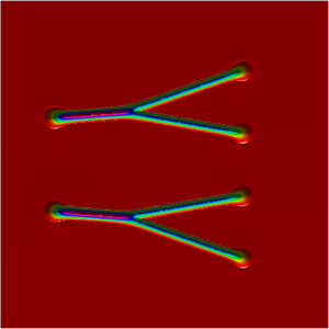
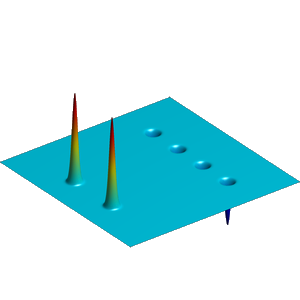
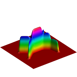
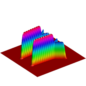
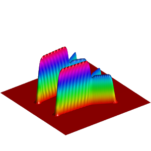
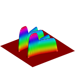
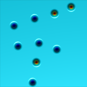
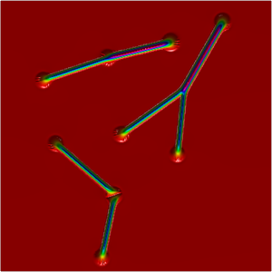
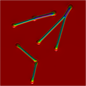
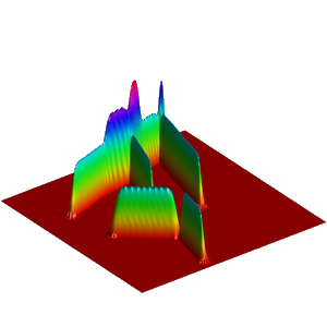
We present below the first results obtained with our simple approach. The following figures are the results of four different experiments with two different values of the parameter  . On the first rows of the figures, we represent two views of the graph of the given density
  . The second rows represent two views of the graph of the norm of the optimal vector field for each value of . As expected, ``Kirchhoff's law is approximatively satisfied'' by the support of the vector field which converges to a one dimensional set. Moreover we observe that two different values of may lead to very different optimal structures.
 |
 |
 |
 |
 |
 |
 |
 |
 |
 |
 |
 |
 |
 |
 |
 |
 |
 |
 |
 |
 |
 |
 |
 |
 |
 |
 |
 |
 |
 |