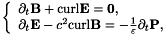
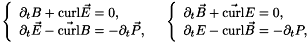
In the semi-classical description of laser-matter interaction, the electromagnetic wave is modelled in a classical way using the Maxwell equations, namely
where we set  and use similar notations for
  and
and  . This system is closed via an expression for the polarization
.
. This system is closed via an expression for the polarization
.
In the framework of classical models for the interaction  is often supposed to be a function of
  and its derivatives. The semi-classical model involves a less phenomenological description of the interaction and matter is described using the quantum mechanical theory via the density matrix formalism. Schematically the density matrix
  is a
is a  complex matrix that describes the states and transitions in matter. Its diagonal elements
  (also called populations) are the probability for an atom to be in the quantum state
  . Only
  states are supposed to be relevant, which means that
 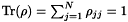 . This fact will be called the trace property in the sequel. The off-diagonal elements
  are called coherences and basically describe transitions between states
and
are called coherences and basically describe transitions between states
and  . The matrix
  is Hermitian and its time evolution is given by the Bloch equations:
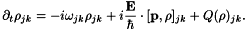
In these equations  where
where  is the energy of the level
. The constant
matrix
is the energy of the level
. The constant
matrix  is the dipole moment matrix. Its coefficients
  are the ability of the transition from
to
to give rise to a contribution to the polarization. The matrix
is Hermitian and its diagonal elements are zero. The commutator
are the ability of the transition from
to
to give rise to a contribution to the polarization. The matrix
is Hermitian and its diagonal elements are zero. The commutator  is defined by
  . Finally
  is a phenomenological relaxation term. The main point is that
 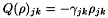 for
for  . We choose the Pauli master equation model for diagonal relaxations, namely
  . Some conditions has to be imposed on the relaxation rates
  and
and  to ensure that
is a positive matrix. In what follows this property has two useful corollaries:
to ensure that
is a positive matrix. In what follows this property has two useful corollaries:  (we recall they are probabilities) and
  * .
* .
To simplify expressions we will denote by  the relaxation-nutation operator given by
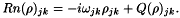
Thus the Bloch equations simply read
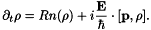
Finally the Bloch equations are coupled to the Maxwell equations, writing the polarization

where  is the atom density.
For the mathematical study and also numerical simulations of this system we use dimensionless equations. Our choice for characteristic values for the different quantities is guided by specific applications where the intensity of the field is high. This may be accounted for by the fact that the Rabi frequency  (where
  and
and  are characteristic values for
and
respectively) is of the same order as the transition frequencies in atoms. We use this Rabi frequency to obtain dimensionless frequencies, times, and relaxation coefficients. Space and magnetic fields are treated taking into account the light velocity in the vacuum. The density matrix elements remain untouched since they are already dimensionless and of order one.
are characteristic values for
and
respectively) is of the same order as the transition frequencies in atoms. We use this Rabi frequency to obtain dimensionless frequencies, times, and relaxation coefficients. Space and magnetic fields are treated taking into account the light velocity in the vacuum. The density matrix elements remain untouched since they are already dimensionless and of order one.
This procedure is only valid if relaxation rates involve larger time scales than the leading frequency, which is a reasonable hypothesis. Otherwise an asymptotic model that does not take into account coherences (in the first place) should be studied. From now on all variables are dimensionless (but we use the same notation as before) and of order one except one parameter  that occurs in the coupling relation, namely
  . This parameter is typically equal to
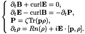
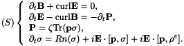
  , which implies that the coupling is not stiff. The dimensionless Maxwell-Bloch equations finally read
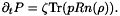
In practice we only have to compute  and not
. The former reads
and not
. The former reads

Now, since numerical simulations nowadays involve only one and two-dimensional models, we give below the precise formulations we use in these contexts. This discussion only concerns the Maxwell equations and the expression of the polarization, since the Bloch equations depend only on space in their coefficients (\textit{via} the electromagnetic field
).
Most numerical simulations involve a one-dimensional model. There is indeed no need for higher dimensions to account adequately for most physical phenomena. To derive a one-dimensional model we first suppose that the unknowns depend only on the time and the space variable  . Therefore the system decouples yielding

In the one-dimensional context a second hypothesis is often imposed, namely  . This leads to the fact that
  and we only consider system (1.3)(b). To simplify notations in this context we will set
  ,
,  ,
,  and
and  . Under this condition formula yields
Since the goal of multi-dimensional simulations is to account for multi-dimensional effects, the second hypothesis for the one-dimensional case is not always relevant. Sometimes two polarization directions, but only a dependence in
, is sufficient to model the physical phenomena. If this is not the case, we may suppose that unknowns only depend on time and the space variables  and
and  , which also decouples the system. Setting
  and
and  with similar notations for the other vector valued variables, we have:
where 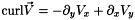 and
and 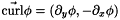 . These two systems describe respectively the transverse electric (TE) and transverse magnetic (TM) modes. They are coupled via the polarization. Indeed
  and
and  are both expressed in terms of
which is computed using
are both expressed in terms of
which is computed using  and
and  .
.
In order to study the nonlinear stability of the numerical schemes, we will need \textit{a priori} estimates that are valid both for the continuous model and the discretized models. For this aim -- and more specifically for  estimates -- we need to express the system in terms of variables that will vanish at infinity. This is the case for the electromagnetic fields, but the trace of the density matrix is one everywhere, so it cannot vanish. The solution to the system
  is the thermodynamic equilibrium state for the Bloch equations. Its off-diagonal elements are zero. Since the diagonal elements of
are zero we may state that
is the thermodynamic equilibrium state for the Bloch equations. Its off-diagonal elements are zero. Since the diagonal elements of
are zero we may state that  . This implies that
will also vanish at infinity. Setting
. This implies that
will also vanish at infinity. Setting  we find that system becomes
This equation may be cast as an equation governing a real vector * valued variable  , where
  (with space dimension
  ),
),
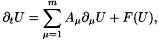
where the matrices  are symmetric and the function
  is a polynomial involving only first and second order monomials and therefore vanishes for
  . Classical arguments from semi-linear hyperbolic theory lead to the following theorem.
Theorem Let  be real and
  , then there exists a time
  such that equation with the Cauchy data
  has a unique solution
  . Moreover this solution is continuous with respect to the initial data.
It is possible to derive
estimates due to cancellations that follow from Lemma below, but such cancellations do not always appear when we consider higher derivatives in the equations.
We now show two estimates for the solutions to system  . They are interesting in themselves but Estimate
  is also used to show the convergence of the numerical schemes
lemma: Let  , then
 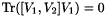 .
.
 estimate for Bloch variables:
Let
be the solution of the Bloch equations, then 
Let us now define the pseudo-energy
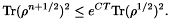
then we have the estimate
estimate for all the variables:
There exists a constant  , that depends only on the matrices
  ,
, on
and the parameter
,
, on
and the parameter  , such that
  .
.
The classical finite difference scheme to discretise the Maxwell-Bloch equations is based the Yee method. This method has the advantage of being non-diffusive, but is dispersive. The coupling we perform here displays the same accuracy limitations as those of the Yee method. It is second order, but not satisfactory for computations over long time intervals. We do not make explicit the space discretization and want to be able to treat complex geometries. What follows does not only apply to the Yee scheme, but also to finite volume formulations that use dual Delaunay-Voronoï meshes. We are not interested in using finite element methods for two reasons: the variational formulation would be different when the form of the relaxation operator
changes for the populations, and the mass matrix would be unnecessarily difficult to invert.
In this method
and
are computed on staggered grids in space and time. We only make the time dependence explicit, since we are interested in the time coupling: given a time step  ,
,  and
and  are the computed values for
  and
and  . The Faraday and Ampère equations are discretized respectively at time
  and
and  by
by
In the sequel we compare different methods for the Bloch equations; these have already been compared in the zero-dimensional case, that is for a forced electromagnetic field. The coupling however leads to new considerations. Indeed the point is now to choose the time of discretization for
. In any case it is natural to take the same space locations as for
for the Yee scheme and the same mesh as
for finite volume approximations.
The literature only uses what we call here strongly coupled methods. The common property for strongly coupled methods is that
is computed at time
and the Bloch equations are written at time
. In both the cases that we present here, the classical Crank-Nicolson scheme reads

The two schemes differ from the expression for the coupling.
In some litterature, the coupling with the Maxwell equations is performed using a value for
at times
and computing
In others, the coupling with the Maxwell equations is done using the formulation  for
for  . The right handside in the Ampere equation reads

In both cases the nonlinear semi-implicit term involving  in the Bloch equation is solved using a predictor-corrector scheme or a fixed-point procedure and couples all the spatial discretization points via the Ampère equation.
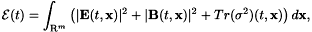
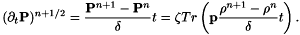
A simple but new way to decouple the Ampere and Bloch equations is to discretise  at time
  . Hence in the Ampère equation the right handside, which we always base on formulation
  , reads
and  has already been computed when we have to evaluate this quantity.
A Crank-Nicolson scheme for the Bloch equations now reads

We still have to perform a fixed-point procedure to solve the Ampère equation in the two- and three-dimensional cases. This is not necessary in the one-dimensional case. Besides at each time step, the Bloch equations associated with each discretization point evolve separately (and are very small systems to invert). They may be computed using a parallel implementation, which is even more useful for two and three-dimensional codes.
Crank-Nicolson schemes have the drawback that they lead to the non-conservation of positiveness properties. For example populations may not remain in the interval  . Nevertheless we may estimate the Bloch variables on a time interval
  . Namely, for example for the weakly coupled Crank-Nicolson scheme, the following lemma holds true.
lemma:
There exist
 and
that depend only on the matrix
, such that for all
and
that depend only on the matrix
, such that for all  and all
  such that
  ,
, 
This estimate will be used in the proof of the convergence for this scheme.
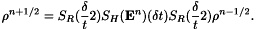
A new scheme for the Bloch equations may be constructed. This handles positiveness problems and is based on a splitting procedure. The main point is that we know how to solve exactly the relaxation-nutation part

and the Hamiltonian part

separately and each part preserves positiveness. Denoting respectively by  and
and  the semi-groups associated to these equations, we obtain a second order scheme by computing
It is both positiveness preserving and decoupled. A second order approximation to  which still ensures positiveness is given in litterature , as well as specific Fadeev Formulae that lead to a very efficient evaluation of this term, which may also be computed on parallel architectures.
In terms of theoretical properties and of efficiency the weakly coupled splitting scheme is the best of all the methods presented here. In particular the equivalent of above Lemma is the physical estimate  . Next we also compare them from the point of view of the quality of the computed solutions.
In this section we show that the weakly coupled Crank-Nicolson scheme and the splitting scheme are both nonlinearly stable under suitable Courant-Friedrichs-Lewy conditions. We suppose that the Yee scheme is implemented on a uniform space grid with mesh step  .
.
theorem:
The weakly coupled Crank-Nicolson and splitting schemes are nonlinearly
Remark:
The CFL condition that follows from the proof of the theorem is not much more restrictive than that of the Yee scheme. Indeed, for the Yee scheme
FOR MORE DETAILS ON THIS ARTICLE SEE, " Time discretizations for maxwell-Bloch equations" of B. Bidégaray.
-stable for  and
and 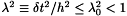 , where
and
, where
and  depend only on the coefficients of the equations.
 should be less than 1 and here we obtain a condition that reads
 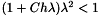 .
.
References
Generated on Wed Mar 17 15:20:18 2004 for C++ Maxwell Bloch GUI Package by
 1.2.18