StochMagnet Core package contains all classes used in the Stoch Magnet module.

The purpose of the code is to simulate the behavior of a ferromagnetic particles with a stochastic perturbation. In the first part , the deterministic part is detailed while in the second part the thermal effect is detailed.

deterministic model

The behavior of ferromagnetic particles submitted is usually modelled by the deterministic dynamical system:

$ \frac{d\mu}{dt}=LL(\mu,H) $

where :

$ LL(\mu,B)=\displaystyle \alpha.\left (\mu \wedge H + \beta \mu \wedge \left ( \mu \wedge H \right ) \right ) $ , the Landau-Lifschitz function
$ \mu $ the magnetic moment
H total magnetic field

In the program the preceeding expression is replaced by

$ LL(\mu,H)=\displaystyle \alpha.\left (\mu \wedge H + \beta \left ( <\mu,H> \mu - |\mu|^2 H \right ) \right ) $

The dedicated class in the SM_LandauLifschitzFunction

The Landau lifschitz equtaion equation can be rewritten as follow :

$ \displaystyle \frac{d\mu}{dt}=\alpha. A(\mu) B $

where $ A: \mathbb{R}^3 \rightarrow M_{3\times3} $ is defined by

$ \displaystyle A(x)=L(x) + \beta ( x.x^t - x^t.x I ) $

and $ L((x_1,x_2,x_3))=\begin{pmatrix}0 & -x_3 & x_2 \\ x_3 & 0 & -x_1 \\ -x_2& x_1 & 0 \end{pmatrix} $

The particles are submitted to

an external field $H_{ext}(t,P_i) $ time and space dependent on the network of P points located at $P_i $
a demagnetized influence from the other particles $H_d(\mu,P_i)$
an exchange interaction between neighbored particles $H_h(\mu)$

The relation of the energy E with respect of the magnetic field H at point $P_i$ and the magnetic moment $\mu_i$ is $\frac{dE}{d\mu}=- H $.

For reference on operators, see the concerning dedicated class :

SM_ZeemanOperator for the Zeeman operator
SM_HeissenbergOperator for the Heissenberg operator
SM_DemagnetizedOperator for the demagnetized operator

Thermal effect

In order to model thermal effects, a stochastic perturbation is introduced. Thermal effect can be embedded in the deterministic system by adding a stochastic perturbation to the field H by considering a standard F-Brownian motion which leads to the following stochastic system

$ \displaystyle d\mu=\alpha. A(\mu_t) H.dt + \epsilon \alpha A(\mu_t)dW_t $

The brownian motion is modelized by the class SM_StochasticFunction and implemented in SMS_BoostNormalFunction.

The noise rate $ epsilon $ is modelized by the SM_NoiseRateFunction a,d is implemented in

Ito approach

The preceeding system is not physically consistent as it does not preserve the norm of $\mu $ which must be invariant equals to 1. To preserve the invariance of the norm of $\mu $, the Ito approach will consist to normalize $\mu $ at each iteration:

$ \displaystyle dY_t=\alpha. A(\mu_t) B.dt + \epsilon_t \alpha A(\mu_t)dW_t $
$ \mu_t=\displaystyle \frac{Y_t}{|Y_t|} $
$ dW_t \sim \sqrt{dt} \mathcal{N}(0,1) $

Stratonovich approach

To preserve the invariance of the norm of $ \mu $, the Ito approach et modified in the Stratonovich approach.

It consists in adding a new term $K_t . dt $ in the equation Ito system and choosing $$K_t$ such that $d|\mu_t|=0 $.

To compute $K_t $, we use the followin Ito Theorem:

Let's denote by $W $ a brownian movement in $R^d $ and

$ \begin{array}{lll} Xt &:& R \rightarrow R^n \\ & & t \mapsto X_t \\ b &:& R^+ \times R^n \rightarrow R^n \\ & & (t,X) \mapsto b(t,X) \\ \sigma &: & R^+ \times R^n \rightarrow R^n\times R^d \\ & & \displaystyle dX_t=b(t,X_t).dt + \sigma(t,X_t) dW_t\\ \end{array} $

if we note by

$ \begin{array}{lll} f &:& R^+ \times R^n \rightarrow R \\ & & (t,x) \mapsto f(t,X)\\ \end{array} $

we have

$ df(t,X_t)=\displaystyle \frac{\partial f}{\partial t} dt + \nabla_xf(X_t).dX_t +\frac{1}{2} \sum_{i,j} \frac{\partial^2 f(t,X_t)}{\partial x_i \partial x_j} .d<x_i,x_j>_t $

with $ d<x_i,x_j>_t=(\sigma(t,X_t).\sigma(t,Y_t>^T)_{ij} dt $

So, we apply the Ito theorem to $f(t,X)=<X,X>$ with $d\mu_t$ verifiing $\displaystyle d\mu_t=\alpha. A(\mu_t) B.dt + \epsilon \alpha A(\mu_t)dW_t + K_tdt$.

$d|\mu_t|^2=2<\mu_t,\alpha.A(\mu_t).B dt+ \epsilon \alpha A(\mu_t)dW_t + K_tdt>+\frac{1}{2}. \sum_{i,j} 2.\delta_{ij}.\varepsilon^2.\alpha^2.A(\mu_t).A(\mu_t)^T dt$

As we have from that $<d\mu_t,\alpha.A(\mu_t).B dt+ \epsilon \alpha A(\mu_t)dW_t>=0 $ , we conclude that

$d|\mu_t|^2=2.<\mu_t,K_t>.dt + \varepsilon^2.\alpha^2 . tr(A(\mu_t).A(\mu_t)^T)dt$

After some computations, we have

$ tr(A(\mu_t).A(\mu_t)^T)=2|\mu_t|^2+3\beta^2|\mu_t|^4-2\beta^2|\mu_t|^4+\beta^2|\mu_t|^4 $

So $ d|\mu_t|^2=\displaystyle 2. \varepsilon^2.\alpha^2.dt.|\mu_t|^2.\left( 1+\beta^2.|\mu_t|^2\right)+2.<\mu_t,K_t>.dt $

To have a null variation of the norm of $\mu$, we can impose that $ K_t= - \varepsilon^2.\alpha^2.dt.|\mu_t|^2.\left( 1+\beta^2.|\mu_t|^2\right) \cdot \mu_t$

So the Ito system becomes with $|\mu_t|=1 $, the Stratonovich system:

$ \displaystyle d\mu_t=\alpha. A(\mu_t) B.dt+ \epsilon \alpha A(\mu_t)dW_t - \varepsilon^2.\alpha^2.\left( 1+\beta^2\right).dt.\mu_t $

We can assume now that the noise rate $\varepsilon $ may be dependant on t. It will be denoted by $ \varepsilon_t $.

Algorithm

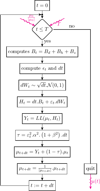
The algorithm is as follow for the stratonovich or Ito algorithm see SM_System class ( $ \tau=0 $ for Ito algorithm)

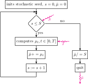
initializes the seed of the stochastic function
initializes to zero, the mean of $ \mu, \bar \mu=0 $
for each trajectory s in [0,S[ do
- initializes $t=0 $
- computes $B=B_z^t+B_h^t+B_d^t $ the Zeeman,Heissenberg and Demagnetized magnetic fields at time t
- computes the time step $dt$ (regular for the version 0.03)
- computes the Brownian motion number $dW_t \sim \displaystyle \sqrt{dt}.\mathcal{N}(0,1) $
- computes $H=B.dt+\varepsilon_t.dW_t$
- computes the normalisation rate $\tau=\varepsilon_t^2.\alpha^2.\left( 1+\beta^2\right).dt $
- computes $\mu_{t+dt}=(1-\tau).\mu_t+LL(\mu_t,H)$
- normalizes $\mu_{t+dt}$ if needed
- loop with new value $t:=t+dt$, $\mu_t:=\mu_{t+dt}$ while $t<T$
The beam simulation, done by the class SM_Beam , can be illustrated as follow:

Whereas the general $\mu_t $ simulation by the Stratonovich system algorithm can be illustrated as follow (see SM_System or SM_StratonovichNormalizedSystem )

3 implementations of systemshave been implemented:

the Ito system by the class SM_ItoSystem
the ususal Stratonovich model SM_StratonovichSystem without normalization of $\mu $ except in the Landau Lifschitz equation where $|\mu|=1 $
the normalized Stratonovich model SM_StratonovichNormalizedSystem with normalization of $\mu$.

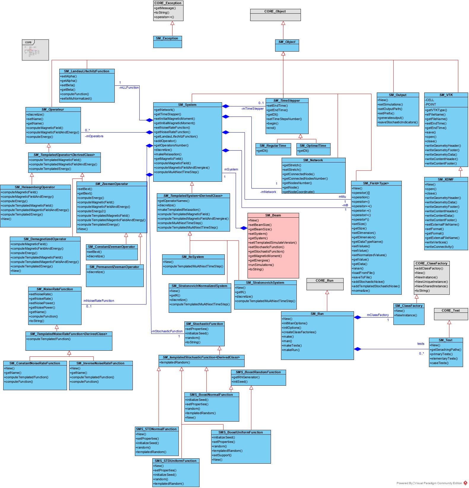
package classes

It contains the generic classes:

SM_Object : the base class of all the classes of the module which implements CORE_Object class
SM_Run : the runner class which implements CORE_Run class
SM_Test : the test class which implements CORE_Test class
SM_Exception : the exception manager of the module which implements CORE_Exception
SM_ClassFactory : the class factory of the modul which implements CORE_ClassFactory

the specific class are :

SM_Beam : to generate the trajectories of a beam which contains :
- SM_StochasticFunction : to generate a random trajectory
- SM_System : the system class which describes to time dependent system to solve
  - SM_LandauLifschitzFunction: the LL calss to compute the LL function
  - SM_Network : the network of the particle
  - SM_TimeStepper : the time step manager class
  - SM_Operator : the map list of operators of the system mapped by its own name
  - SM_NoiseRateFunction : the generic noise rate function
  - SM_Field : the class to describes the real field of size N x D as $B,\mu_0$ The system classes are described with:
SM_TemplatedSystem which implements the SM_System class by templated methods
SM_ItoSystem describes an ITO system and implements the SM_TemplatedSystem class
SM_StratonovichSystem describes a Stratonovich system and implements the SM_TemplatedSystem class
SM_StratonovichNormalizedSystem describes a Stratonovich system by a renormalization of the magnetic moment and implements the SM_TemplatedSystem class

The operators are described by this classes:

SM_TemplatedOperator which implements the SM_Operator class by templated methods
SM_ZeemanOperator describes the Zeeman operator and implements SM_TemplatedOperator
SM_ConstantZeemanOperator describes the constant Zeeman field operator a
SM_PermanentZeemanOperator describes the permanent Zeeman field operator
SM_ZeemanOperator describes an external magnetic field depending on time and particules.
SM_DemagnetizedOperator describes the demagnetized operator and implements SM_TemplatedOperator
SM_HeissenbergOperator describes the exchange operator and implements SM_TemplatedOperator

The stochastic functions are described by this class:

SM_TemplatedStochasticFunction which implements the SM_StochasticFunction class by templated methods
SMS_BoostNormalFunction describes a stochastic function modeled by the Boost Normal Law
SMS_BoostUniformFunction describes a stochastic function modeled by the Boost Uniform Law
SMS_STDNormalFunction describes a stochastic function modeled by the C-Standart Normal Law
SMS_STDUniformFunction describes a stochastic function modeled by the C-Standart Uniform Law

The noise rate functions are described by this classes:

SM_TemplatedNoiseRateFunction which implements the SM_NoiserateFunction by templated methods
SM_ConstantNoiseRateFunction describes a constant noise rate and implements SM_TemplatedNoiseRateFunction
SM_InverseNoiseRateFunction describes an inverse noise rate and implements SM_TemplatedNoiseRateFunction

The result of the program are managed by the classes:

SM_VTK the VTK interface class
SM_XDMF the XDMF class which is an implementation of the SM_VTK interface

The organization of this package is as follow: